들어가며
AI수업이 오늘을 포함해서 이제 2번 밖에 남지 않았다. NVIDIA 엠버서더이신 교수님께서 NVIDIA 공인교육 과정 중 하나인 딥러닝 기초에 대해 수업을 해주실텐데 어떤 내용이 있었는지 복기해보자.
실습 환경
JupyterLab에서 진행이 되고, GPU메모리를 지워야하는 경우에는 아래 코드를 실행함으로써 모두 지워준다.
import IPython
app = IPython.Application.instance()
app.kernel.do_shutdown(True)
MNIST 데이터 세트로 이미지 분류
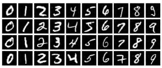
먼저 MNIST를 위한 Keras 데이터 세트를 로드해 보자. 그리고 훈련 데이터와 검증 데이터로 나누어 각각 할당해준다.
from tensorflow.keras.datasets import mnist

# the data, split between train and validation sets
(x_train, y_train), (x_valid, y_valid) = mnist.load_data()
불러온 데이터를 `shape`로 확인하고, `dtype`으로 데이터의 타입을 확인한다. 28 x 28 이미지가 0~255의 양의 정수 값으로 표현된 것을 알 수 있다. 0은 검은색, 255는 흰색이다.
x_train.shape # (60000, 28, 28)
x_valid.shape # (10000, 28, 28)

x_train.dtype # dtype('uint8')
x_train.min() # 0
x_train.max() # 255
학습 및 검증 데이터들을 28 x 28 = 784개의 연속 픽셀로 이루어진 단일array로 `reshape`해준다. 이미지 평탄화라고도 한다.
x_train = x_train.reshape(60000, 784)
x_valid = x_valid.reshape(10000, 784)
딥러닝 모델은 0에서 1 사이의 부동 소수점 수를 처리하는데 뛰어나다. 따라서 정규화 과정을 진행한다.
x_train = x_train / 255
x_valid = x_valid / 255
범주 인코딩
범주 특성을 알 수 있는 표현으로 변환하는 것을 말한다. 여기서는 0 또는 1의 바이너리 값을 사용하여 표현할 수 있다.

모델 생성 및 트레이닝
- 어느 정도 예상되는 형식으로 데이터를 수신하는 입력 레이어
- 각각 다수의 뉴런으로 구성된 여러 개의 숨겨진 레이어 각 뉴런은 가중치로 네트워크의 추측에 영향을 미칠 수 있으며, 가중치는 네트워크가 수많은 반복을 통해 성능에 대한 피드백을 수신하고 학습하면서 업데이트하게 되는 값
- 주어진 이미지에 대한 네트워크의 추측을 보여주는 출력 레이어
from tensorflow.keras.models import Sequential
from tensorflow.keras.layers import Dense

# 모델 인스턴스화
model = Sequential()

# 입력 레이어 생성
model.add(Dense(units=512, activation='relu', input_shape=(784,)))

# 은닉 레이어 생성
model.add(Dense(units = 512, activation='relu'))

# 출력 레이어 생성
model.add(Dense(units = 10, activation='softmax'))

# 모델 요약 및 컴파일
model.summary()
model.compile(loss='categorical_crossentropy', metrics=['accuracy'])

# 모델 트레이닝
history = model.fit(
    x_train, y_train, epochs=5, verbose=1, validation_data=(x_valid, y_valid)
)
정확도 관찰
5회의 에포크 각각에 대해 `accuracy` 및 `val_accuracy` 점수를 확인한다. `accuracy`는 모든 훈련 데이터에 대한 에포크 동안의 모델 성능이 어땠는지를 명시한다. `val_accuracy`는 모델을 트레이닝하는 데 전혀 사용되지 않는 검증 데이터에 대한 모델 성능이 어땠는지를 나타낸다.
미국 수화 데이터세트 이미지 분류
26개의 문자가 포함되어있고, 이 중 두개의 문자 (j, z)에는 동작이 요구되기 때문에 훈련 데이터셋에 포함되지 않았다.

데이터 시각화
import matplotlib.pyplot as plt
plt.figure(figsize=(40,40))

num_images = 20
for i in range(num_images):
    row = x_train[i]
    label = y_train[i]

    # 1D 모양의 784개 픽셀을 2D 모양의 28x28으로 재구성
    image = row.reshape(28,28)
    plt.subplot(1, num_images, i+1)
    plt.title(label, fontdict={'fontsize': 30})
    plt.axis('off')
    plt.imshow(image, cmap='gray')
모델 트레이닝

모델의 훈련 정확도는 높지만 검증 정확도는 훈련 정확도만큼 높지 않다. 그 이유는 학습된 데이터에 대해서는 이해를 잘하고 있지만 새로운 데이터에 대해서는 이해도가 낮기 때문이다. 이러한 현상을 과적합이라고 한다.
CNN(합성곱 신경망)
from tensorflow.keras.models import Sequential
from tensorflow.keras.layers import (
    Dense,
    Conv2D,
    MaxPool2D,
    Flatten,
    Dropout,
    BatchNormalization,
)
# 모델 인스턴스화
model = Sequential()

# 2D 컨벌루션 레이어
model.add(Conv2D(75, (3, 3), strides=1, padding="same", activation="relu",
                 input_shape=(28, 28, 1)))
# 배치 정규화
model.add(BatchNormalization())

# MaxPooling 2D 레이어
model.add(MaxPool2D((2, 2), strides=2, padding="same"))

# 2D 컨벌루션 레이어
model.add(Conv2D(50, (3, 3), strides=1, padding="same", activation="relu"))
model.add(Dropout(0.2))
model.add(BatchNormalization())
model.add(MaxPool2D((2, 2), strides=2, padding="same"))
model.add(Conv2D(25, (3, 3), strides=1, padding="same", activation="relu"))
model.add(BatchNormalization())
model.add(MaxPool2D((2, 2), strides=2, padding="same"))
model.add(Flatten())
model.add(Dense(units=512, activation="relu"))
model.add(Dropout(0.3))
model.add(Dense(units=num_classes, activation="softmax"))
| Conv2D | 작은 커널은 입력 이미지들을 훑으며, 분류에 중요한 특징들을 파악 |
| BatchNormalization | 은닉층들의 값을 스케일링하여 학습을 개선 |
| MaxPool2D | 이미지를 가져와서 더 낮은 해상도로 축소, 모델이 약간의 변화에 더욱 견고하게 만들 수 있고, 모델의 학습 및 추론을 더욱 빠르게 할 수 있음 |
| Dropout | 과적합을 방지하는 기술 |
| Flatten | 다차원 입력을 1차원으로 변환 |
| Dense | * 첫번째 dense레이어는 특징벡터를 입력으로 받으며, 어떠한 특징이 분류에 기여하는 지 학습 * 두번째 dense레이어는 우리의 분류 예측 결과를 위한 마지막 레이어로 활용 |
Assessment
신선한 과일과 썩은 과일을 인식하도록 모델을 트레이닝해보자.
ImageNet 기본 모델 로드
사전 트레이닝된 모델로 시작 `VGG16`
from tensorflow import keras

base_model = keras.applications.VGG16(
    weights='imagenet',
    input_shape=(224, 224, 3),
include_top=False)기본 모델 동결
ImageNet 데이터 세트에서 학습된 모든 내용이 초기 트레이닝에서 손상되지 않도록 하기 위함이다.
# Freeze base model
base_model.trainable = False모델에 레이어 추가
레이어를 사전 트레이닝된 모델에 추가한다.
# Create inputs with correct shape
inputs = keras.Input(shape=(224, 224, 3))

x = base_model(inputs, training=False)

# Add pooling layer or flatten layer
x = keras.layers.GlobalAveragePooling2D()(x)

# Add final dense layer
outputs = keras.layers.Dense(6, activation = 'softmax')(x)

# Combine inputs and outputs to create model
model = keras.Model(inputs, outputs)

model.summary()

모델 컴파일
손실 및 지표 옵션으로 모델을 컴파일한다.
model.compile(loss = 'categorical_crossentropy' , metrics = ['accuracy'])
데이터 증강
from tensorflow.keras.preprocessing.image import ImageDataGenerator

datagen = ImageDataGenerator(
    rotation_range=10,  # randomly rotate images in the range (degrees, 0 to 180)
    zoom_range=0.1,  # Randomly zoom image
    width_shift_range=0.1,  # randomly shift images horizontally (fraction of total width)
    height_shift_range=0.1,  # randomly shift images vertically (fraction of total height)
    horizontal_flip=True,  # randomly flip images horizontally
    vertical_flip=True, # Don't randomly flip images vertically
)
데이터세트 로드
# load and iterate training dataset
train_it = datagen.flow_from_directory('data/fruits/train/',
                                       target_size=(224,224),
                                       color_mode='rgb',
                                       class_mode="categorical")
# load and iterate validation dataset
valid_it = datagen.flow_from_directory('data/fruits/valid/',
                                      target_size=(224,224),
                                      color_mode='rgb',
                                      class_mode="categorical")
모델 트레이닝
model.fit(train_it,
          validation_data=valid_it,
          steps_per_epoch=train_it.samples/train_it.batch_size,
          validation_steps=valid_it.samples/valid_it.batch_size,
          epochs=10)
파인튜닝을 위해 모델 동결 해제
이미 92%의 검증 정확도에 도달한 경우 이 단계는 선택사항이다. 92%에 도달하지 않은 경우에는 매우 낮은 학습률로 모델을 파인튜닝 할 것을 권장한다.
# Unfreeze the base model
base_model.trainable = True

# Compile the model with a low learning rate
model.compile(optimizer=keras.optimizers.RMSprop(learning_rate = .00001),
              loss = 'categorical_crossentropy' , metrics = ['accuracy'])

model.fit(train_it,
          validation_data=valid_it,
          steps_per_epoch=train_it.samples/train_it.batch_size,
          validation_steps=valid_it.samples/valid_it.batch_size,
          epochs=20)
모델 평가
정확도 약 98%로 기준치를 달성했다.
model.evaluate(valid_it, steps=valid_it.samples/valid_it.batch_size)
평가 실행
평균 정확도 98%로 과제 수행 기준을 달성하게 되었다.
from run_assessment import run_assessment
run_assessment(model, valid_it)
마무리
과제라고해서 많이 어려울 것이라 생각했지만 예제 파일을 참고함으로써 어떤 기능이 어떠한 역할로 적용이 되었는지를 이해하면서 대입을 하니까 생각보다 괜찮았다. NVIDIA 공식 수료증까지 발급이 돼서 동기부여도 되는 것 같다.
'ABC부트캠프 테크노트' 카테고리의 다른 글
| [29일차] ABC부트캠프 : 데이터 라벨링 (0) | 2024.08.13 |
|---|---|
| [28일차] ABC부트캠프 : NVIDIA 트랜스포머 기반 NLP 애플리케이션 구축 (0) | 2024.08.12 |
| [26일차] ABC부트캠프 : 미니프로젝트 발표 (0) | 2024.08.08 |
| [25일차] ABC부트캠프 : 미니 프로젝트 준비 (0) | 2024.08.07 |
| [24일차] ABC부트캠프 : 딥러닝3 (0) | 2024.08.06 |