들어가며
간단한 데이터 전처리 과정 진도를 모두 마치고, 교수님께서 설계하신 미니 프로젝트를 진행해보았다. 지금까지 배운 전처리 방법들을 활용해서 조건에 맞게 데이터를 추출해보자.
1. 데이터 불러오기
주어진 csv파일 `아파트(매매)_실거래가_서울_2022.csv`를 활용하여 데이터프레임을 생성하고 `df_trade`변수에 저장한 후 아래의 결과를 확인 (파일의 내용을 확인하여 불필요한 데이터는 제외하고 데이터프레임을 만들어야함)
- `df_trade`에 저장된 데이터프레임의 전체 관측치(행)와 변수(열)의 개수 출력
- `df_trade`에 저장된 데이터프레임의 변수(열) 별 데이터유형을 확인 및 출력
먼저 csv파일을 열어서 어떤 식으로 구성되어 있는지 살펴보았다. 상단의 16줄이 파일에 대한 설명으로 자리하고 있었다. 데이터프레임을 생성하기 위해서는 불필요한 부분을 제외해야 하므로, `skiprows=16`을 지정해주었다. 그리고 한글이 포함된 데이터파일이기 때문에 `encoding='CP949'`도 함께 지정했다.

파일 경로를 지정해줄 때 마크다운에 있는 파일이름을 복사해서 붙여넣었는데 파일을 찾을 수 없다는 오류가 떴었다. 이런 오류가 떴던 교육생 분들이 적잖게 있었는데, 교수님께서는 마크다운에 있는 문자의 코드 값이 다르게 인식될 수 있어서 이런 오류가 뜰 수 있다고 하셨다. 그래서 마크다운에 있는 파일이름을 복사하지 않고 직접 입력함으로써 문제를 해결했다.
import pandas as pd

df_trade = pd.read_csv("./아파트(매매)_실거래가_서울_2022.csv", encoding='CP949', skiprows=16)
df_trade
데이터프레임을 생성한 후, 각 변수별 데이터타입을 확인하기 위해 `dtypes`메서드를 사용했다.
df_trade.dtypes
2. 결측값 및 파생 변수 생성
위 1번의 `df_trade`의 데이터프레임에 선택조건의 관측치(행)만을 선택하여 `df_trade`에 저장한 후 `평당거래금액(만원)`변수(열)를 추가하고 `df_trade`데이터프레임을 출력
- 선택조건 : `해제사유발생일`이 결측값인 데이터 (결측값이 아닌 경우 취소된 거래 건)
- 산술식 : `평당거래금액(만원) = 거래금액(만원) / 전용면적( ㎡ )`
선택조건이 `해제사유발생일`이 결측값 즉, `NaN`인 값을 선택해야하므로 결측치인지 아닌지 판단해주는 `isnull()`메서드를 사용할 수 있다. `cond` 변수에 저장하고 출력해보면 아래와 같이 논리값이 할당된 것을 알 수 있다.

이제 `cond`에서 True인 값에 산술식의 결과값을 대입해준다. 여러가지 방법이 있지만 여기서는 `loc`를 이용하여 `평당거래금액(만원)` 변수 생성과 동시에 산술식 결과값을 각 행에 저장했다.
df_trade.loc[cond, '평당거래금액(만원)'] = df_trade['거래금액(만원)'] / df_trade['전용면적(㎡)']
df_trade
3. 데이터 집계 및 부분선택
위 2번의 `df_trade`의 데이터프레임을 대상으로 `시군구`별 `평당거래금액(만원)`의 평균이 높은 5개 지역을 `target`으로 지정한 후 아래의 결과를 확인
- `df_trade`데이터프레임의 관측치(행) 중 `시군구`변수가 `target`에 속하는 관측치만을 선택하여 출력
- `df_trade`데이터프레임의 관측치(행) 중 `거래유형`이 `중개거래`인 관측치만을 선택하여 출력
- 위 2개의 조건을 모두 만족하는 관측치(행)를 선택하고 `df_sub`변수에 결과를 저장
먼저 `시군구`별로 집계를 해야 하므로 `groupby()`를 사용한다. 첫번째 매개변수에 대상 변수인 `시군구`를 지정하고, `시군구`를 인덱스로 사용하지 않기 때문에 `as_index`에는 False를 지정한다. 그 다음 `평당거래금액(만원)` 변수를 선택하고 `mean()`메서드로 마무리한다. 이 결과값을 `df_trade1`이라는 변수에 저장하고 출력해보면 299개의 `시군구`별로 `평당거래금액(만원)`의 평균값을 확인할 수 있다.
df_trade1 = df_trade.groupby('시군구', as_index=False)['평당거래금액(만원)'].mean()
그 다음 이 `df_trade1`를 이용해서 평균값 상위 5개를 구한다. 이 부분은 `nlargest()`메서드를 사용할 수 있다.
target = df_trade1.nlargest(5, '평당거래금액(만원)')
target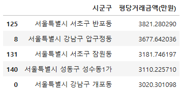
원본 데이터프레임인 `df_trade`에서 `시군구`를 선택한 후, 이 값이 이전에 구한 평균값 상위 5개에 속하는 지 판단한다. `cond1`변수에 할당한 후 True에 해당하는 관측치를 출력하면 다음과 같다.
cond1 = df_trade['시군구'].isin(target['시군구'])
df_trade[cond1]
이제 `df_trade`의 `거래유형` 값이 `중개거래`와 같은 관측치를 선택하는 부분이다. 10733개의 상당히 많은 관측치가 조건에 해당하는 것을 알 수 있다. `중개거래`가 아닌 값들은 대부분 `직거래`로 확인됐다.
cond2 = df_trade['거래유형'] == '중개거래'
df_trade[cond2]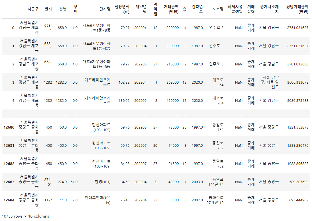
이제 위의 조건 `cond1`과 `cond2`에 모두 해당되는 관측치를 선택한다. `&`연산자를 사용해서 두 조건 모두 참일 경우를 선택할 수 있다. 해당되는 조건의 관측치를 `df_sub`변수에 다시 저장하고 출력해보면 다음과 같이 381개의 관측치로 추려지는 것을 확인할 수 있다.
cond3 = cond1 & cond2
df_sub = df_trade[cond3]
df_sub
4. 데이터 집계 및 데이터 처리 2
위 3번의 `df_sub`의 데이터프레임을 대상으로 `단지명`별 `거래건수`, `평당평균거래금액(만원)`, `최대거래금액(만원)`, `최소전용면적(㎡)`을 집계한 후 아래의 조건에 따른 15개 관측치(행)을 선택하여 `df_result`에 저장한 후 결과를 확인
- 선택 조건 : `거래건수`가 많은 15개의 관측치 선택 (`거래건수`가 동일할 경우 `평단평균거래금액(만원)`이 높은 순)
- 출력 변수 : `단지명`, `거래건수`, `평당평균거래금액(만원)`, `최대거래금액(만원)`, `최소전용면적(㎡)`
일단 `단지명`별로 집계를 해야하기 때문에 `groupby()`를 사용한다. 그리고 `agg()`를 이용하여 각 변수를 집계 종류에 따라 딕셔너리로 지정해준다.
| 집계에 사용할 변수 | 집계 유형 |
| `단지명` | `count` : 단지명으로 거래건수 계산 |
| `평당거래금액(만원)` | `mean` : 평당거래금액의 평균값 계산 |
| `거래금액(만원)` | `max` : 거래금액의 최대값을 계산 |
| `전용면적(㎡)` | `min` : 전용면적의 최소값을 계산 |
df_sub2 = df_sub.groupby('단지명').agg({'단지명':'count', '평당거래금액(만원)':'mean','거래금액(만원)':'max', '전용면적(㎡)':'min'})
df_sub2
값이 의미하는 바를 변수이름으로 지정해주기 위해 기존의 변수이름을 `rename()`을 이용하여 수정해준다.
df_sub2 = df_sub2.rename(columns={'단지명':'거래건수', '평당거래금액(만원)':'평당평균거래금액(만원)', '거래금액(만원)':'최대거래금액(만원)', '전용면적(㎡)':'최소전용면적(㎡)'})
df_sub2
마지막으로 `거래건수` 상위 15개의 값을 추출하기 위해 `sort_values()`를 사용한다. `nlargest()`를 사용할 수도 있지만, 조건에 "`거래건수`가 동일할 경우 `평단평균거래금액(만원)`이 높은 순" 이 명시되어 있기 때문에 `sort_values()`가 이러한 부분을 처리해줄 수 있다. 첫번째 매개변수에 리스트형태로 `거래건수`와 `평당평균거래금액(만원)`을 넘겨준다. `ascending`옵션에는 넘겨준 변수 순서에 맞춰 False를 지정해줌으로써 내림차순으로 정렬한다.
df_result = df_sub2.sort_values(['거래건수', '평당평균거래금액(만원)'], ascending=[False, False]).head(15)
df_result
5. 데이터프레임 저장
위 4번의 `df_result` 데이터프레임을 `agg_result.csv`이름의 파일로 저장
`to_csv()`메서드를 사용해서 첫번째 매개변수에 경로와 파일이름을 지정해주고, `단지명`을 인덱스로 사용하기 위해 `index`옵션을 True로 지정한다. 또한 데이터프레임에 한글이 포함되어있기 때문에 `encoding`을 CP949로 지정한다.
df_result.to_csv('./agg_result.csv', index=True, encoding='CP949')
저장된 `agg_result.csv`을 열어보면 아래와 같이 csv파일 형식으로 잘 저장된 것을 확인할 수 있다.

마무리
지금까지 배웠던 많은 메서드, 함수들을 조건에 맞게 쓰려고 하니까 쉽지 않았다. 꼭 한가지 방법에만 매몰되기보다는 여러 방법들을 같이 적용해보면서 문제를 바라보는 시야를 넓혀가는게 좋을 것 같다.
그리고 지금까지 파이썬 기초랑 데이터분석 기초를 강의해주신 교수님께 정말 감사하다는 말씀을 드리고 싶다. 내일부터는 새로운 교수님께서 강의를 해주시니 나는 수업내용들을 잘 받아먹을 준비를 해야겠다.
'ABC부트캠프 테크노트' 카테고리의 다른 글
| [12일차] ABC부트캠프 : ESG포럼 & 세미나2 (0) | 2024.07.19 |
|---|---|
| [11일차] ABC부트캠프 : 랭킹뉴스 크롤링 및 데이터 시각화 (0) | 2024.07.18 |
| [9일차] ABC부트캠프 : 파이썬 프로그래밍 데이터 집계 및 처리 심화 (0) | 2024.07.16 |
| [8일차] ABC부트캠프 : 파이썬 프로그래밍 데이터 전처리 & 시각화 (2) | 2024.07.16 |
| [7일차] ABC부트캠프 : 파이썬 프로그래밍 데이터 전처리 기초 (0) | 2024.07.12 |